In this article, I introduce the Markov chain Monte Carlo from a non-technical perspective, often referred to simply as MCMC. MCMC is widely used in Bayesian statistical model fitting. MCMC has many different methods. Here I will mainly introduce the Metropolis–Hastings algorithm. For the sake of brevity, I will ignore some details. I highly recommend that you read the [BAYES] manual before practicing MCMC.
We continue with the previous article Bayesian statistics introduced Part 1: The coin-throwing example mentioned in the basic concepts. We are interested in the posterior distribution of the parameter θ, which is the probability that the "head" is on the top when the coin is thrown. Our prior distribution is flat, with no information Beta distribution parameters 1 and 1. Then we will use the binomial likelihood function to quantify our experimental data, throwing the coin four times with "heads" up. We can use MCMC's MH algorithm to generate a posterior distribution of θ samples. This sample can then be used to estimate problems such as the mean of the posterior distribution.
There are three basic parts of this technology:
1. Monte Carlo
2. Markov chains
3. M–H algorithm
Monte Carlo methods
Monte Carlo refers to the method of generating pseudo-random numbers (referred to as pseudo-random numbers). Figure 1 illustrates some of the features of Monte Carlo experiments.
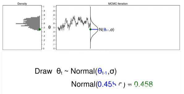
Figure 1: Proposal distributions, trace plots, and density plots
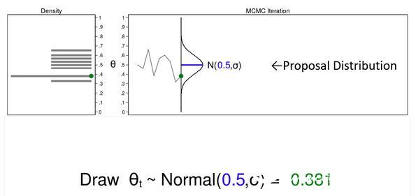
In this example, I will generate a series of random numbers from the mean 0.5 and arbitrary variance σ of the normal distribution. The normal distribution is called the recommended distribution.
The upper right corner of the figure is called a trajectory plot, which shows the θ value according to the drawing order. It also shows that the recommended distribution rotates 90 degrees clockwise, and I will shift it to the right each time I draw a θ value. The green dot trace shows the current value of θ.
The density plot in the upper left corner is a histogram sample rotated 90 degrees counterclockwise. I rotated the axis so that the θ axis is parallel. Similarly, the green dot density plot shows the current value of θ.
Let's draw 10,000 θ random values ​​to see how it works.
Animation 1: A Monte Carlo experiment
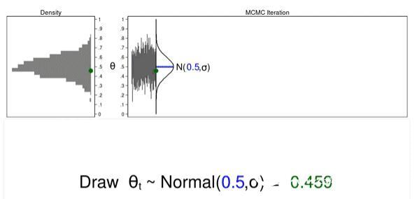
Animated Figure 1 illustrates several important features. The first suggestion is that the distribution will not change from one iteration to another. Second, as the sample size increases, the density map looks more and more like the proposed distribution. Third, the trajectory map is stationary - all iterative variables, the variations appear to be the same.
The sample generated by the Monte Carlo simulation looks like a suggested distribution, and many times it is exactly what we need. However, we need an additional tool to generate a sample from the posterior distribution.
Markov chain Monte Carlo methods
The Markov chain is a sequence of numbers, each number depending on the previous number in the sequence. For example, we plot the θ value from a normal suggested distribution and the previous value with an average equal to θ. Figure 2 shows the trajectory plot and the density plot. The current θ value (θt=0.530) is plotted from a proposed distribution (θt−1=0.712) with an average value equal to the pre-θ value.
Figure 2: A draw from a MCMC experiment
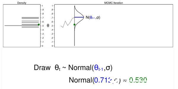
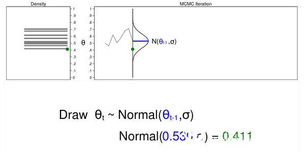
Figure 3 below shows the trajectory map and density map for the next iteration in the sequence. The mean value of the proposed density is now θt−1 = 0.530, and we have plotted the random value θt=0.411 from the new proposed distribution.
Figure 3: The next iteration of the MCMC experiment
Let's use MCMC to draw 10,000 θ random values ​​to see how it works.
Animation 2: A MCMC experiment
Animated Figure 2 shows the direct difference between the Monte Carlo and MCMC experiments. First, the proposed distribution varies with each iteration. This generates a trajectory map of random walk patterns: all iterations are not the same. Second, the resulting density map does not look like the proposed distribution or any other useful distribution, and certainly not a posterior distribution.
The reason that the MCMC failed to obtain the sample from the posterior distribution is that we have not input any posterior distribution information in the process of generating the sample. We can increase the sample by keeping the θ value, which is more likely to be the value under the posterior distribution and less likely to be the discarded value.
However, based on the posterior distribution, the most obvious difficulty in accepting and rejecting the recommended value of θ is that we usually do not know the form of the function of the posterior distribution. If we know its function form, we can directly calculate the probability without generating a random sample. So how can we accept or reject the proposed θ value without knowing the form of the function? The answer is the MH algorithm!
MCMC and M–H algorithms
The MH algorithm can be used to determine whether to accept the θ-suggested value if we do not know the form of the posterior distribution function. Let us divide the MH algorithm into several steps and then go through several iterations to see how it is implemented.
Figure 4: MCMC with the M–H algorithm: Iteration 1
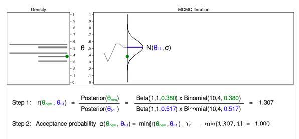
Figure 4 shows the proposed distribution trace and density map equal to (θt−1=0.0.517). We have already plotted an estimate θ (θnew=0.380). I define this value as θnew because we have not yet determined whether we want to use this value.
We use the MH algorithm to calculate the ratio from step 1.
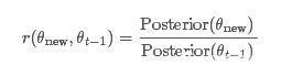
We do not know the functional form of the posterior distribution, but in this case we can replace the product of the prior distribution and the likelihood function. The calculation of ratios is not all that simple, but we can make things easier.
Step 1 in Figure 4 shows that the posterior probability ratio of (θnew=0.380) and (θt−1=0.0.517) is equal to 1.307. Step 2 We calculate the acceptance probability α(θnew, θt−1), which is the lowest ratio r(θnew, θt -1) and 1. Step 2 is necessary because the ratio must be between 0 and 1.
The acceptance probability is equal to 1, so we accept (θnew=0.380) and the average of the proposed distribution becomes 0.380 in the next iteration.
Figure 5: MCMC with the M–H algorithm: Iteration 2
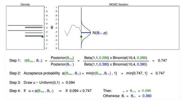
Figure 5 shows that the next iteration (θnew=0.286) is based on a posterior distribution with an average value of (θt−1=0.380). step 1
The calculated ratio r(θnew, θt−1) is equal to 0.747, which is less than 1. The acceptance probability α (θnew, θt−1) calculated in step 2 is equal to 0.747.
We do not automatically reject θnew because the acceptance probability is less than one. Instead, we can plot the random number U from the uniform distribution (0, 1) in step 3. If U is less than the acceptance probability, we accept the recommended value θnew. Conversely, we reject θnew and leave θt−1.
Here u=0.094 is less than the acceptance probability (0.747), so we accept (θnew=0.286). I show θnew and 0.286 in green in Figure 5 that they have been accepted.
Figure 6: MCMC with the M–H algorithm: Iteration 3
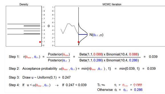
Figure 6 shows that the next iteration (θnew=0.088) is based on a posterior distribution with an average value of (θt−1=0.286). The ratio r (θnew, θt−1) calculated in step 1 is equal to 0.039, which is less than 1. The acceptance probability α (θnew, θt−1) calculated in step 2 is equal to 0.039. The value of U calculated in step 3 is 0.247, which is greater than the acceptance Probability. So in step 4, we reject θnew=0.088 and leave θt−1=0.286.
Let's use the MCMC of the MH algorithm to draw 10,000 random values ​​of θ to see how it works.
Animation 3: MCMC with the M–H algorithm
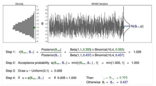
Animated Figure 3 shows several issues. First, the proposed distribution will change with most iterations. It should be noted that if θnew is accepted, they will be shown in green and if they are rejected they will be shown in red. Second, when we only use the MCMC, the trajectory plot does not show a random walk pattern, and the changes in all iterations are similar. Finally, the density map looks like a useful distribution.
Rotate the density map results for a closer look.
Figure 7: A sample from the posterior distribution generated with MCMC with the M–H algorithm
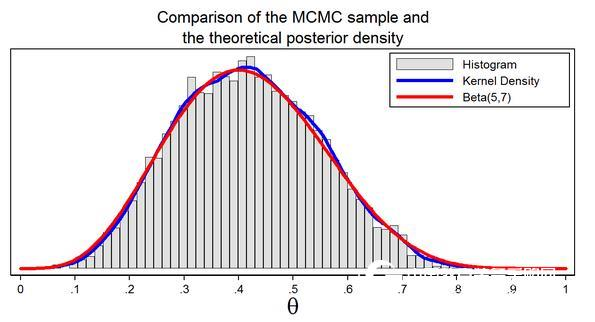
Figure 7 shows our sample histogram generated using the MCMC MCMC. In this example, we know that the parameters of the posterior distribution are Beta 5 and 7. The red line shows the posterior distribution analysis, and the blue line is the nuclear density map of the sample. The nuclear density map is similar to the Beta(5,7) distribution, which shows that our sample is a good approximation of the theoretical posterior distribution.
We can use samples to calculate the mean or median of the posterior distribution, the probability of a 95% confidence interval, or the probability of θ falling in any interval.
MCMC and MH Algorithms in Stata
Let's go back to the example of throwing a coin using bayesmh. With binomial possibilities, we specify a beta distribution parameter 1 and 1.
Example 1: Using bayesmh with a Beta(1,1) prior
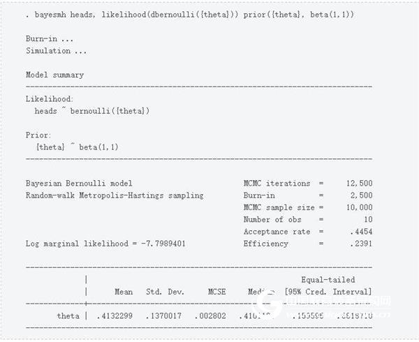
The output tells us that Bayesmh had completed 12,500 MCMC iterations. "Burn-in" tells us that in order to reduce the influence of random starting values ​​in the chain, 2500 of the iterations are discarded. The following line tells us that the final MCMC sample size is 10,000, and the next line shows that our dataset has 10 observations. The acceptance probability θ recommendation ratio is included in the final MCMC sample. I recommend that you read the Stata Bayesian Analysis Reference Manual and understand the definition of efficiency, but high efficiency indicates low autocorrelation and low efficiency indicates high autocorrelation. The Monte Carlo standard error (MCSE) is displayed in the coefficient table to estimate the approximate error of the posterior mean.
Check the convergence of the chain
The word "convergence" has a different meaning in the expression of MCMC and maximum likelihood. The algorithm for maximum likelihood estimation is iterated until it converges to its maximum. The MCMC chain does not iterate until the best value is determined. The outer chain simply iterates until the required sample size is reached and any algorithm stops. In fact, the out-of-service chain does not indicate the generation of the best sample in the posterior distribution. We must check the sample to stop the problem from appearing. We can use the bayesgraph diagnostics graphical form to examine the sample.
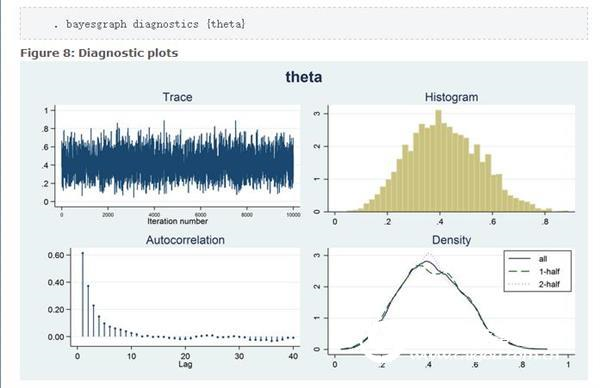
Figure 8 shows a diagnostic plot and a correlegram of the trajectory, histogram, and density plots containing MCMC samples. The trajectory has a smooth pattern, which is exactly what we want to see. The random walk pattern in Figure 2 shows the problem with the chain. Histograms do not have any special features such as multiple modes. The complete sample nuclear density map, the first half of the chain, and the latter half of the chain all look very similar and do not have any special features such as different densities in the first and second half of the chain. The Markov chain is used to generate samples and produce an autocorrelation, but the autocorrelation decreases rapidly with larger lag values. These figures do not indicate any problems with our sample.
to sum up
This article describes the idea behind using the MH algorithm MCMC. Please note that I have omitted some details and have omitted some of the assumptions to make things easier and move forward with our feelings. Stata's bayesmh command actually implements a more difficult algorithm, which we call an adaptive MCMC with MH algorithm. But the basic concept is the same, and I hope to give you some inspiration.
Height Adjustable Desk helps create a healthier work environment by allowing you to move throughout your day. Switching between sitting and standing throughout a long workday provides several health benefits for the body, such as increased blood flow and enhanced posture. Standing throughout the day also keeps the mind alert and productive while you work.
Fast lifting, lifting speed up to 32mm / s, Uniform and stable, cup water balance, double motor balanced drive, lifting the whole table without shaking. The rising and falling sound is less than 45 dB, which is lower than that of keyboard typing.
Adjustable Office Desk,Foldable Computer Adjustable Desk,Electric Adjustable Office Desk,Electric Adjustable Standing Desk
CHEX Electric Standing Desk , https://www.chexdesk.com